
Introdução
Dando continuidade à primeira parte desta série, iremos implementar alguns dos algoritmos apresentados anteriormente com as ferramentas que instalamos em outros posts.
Algoritmo 1: Threshold
Para implementar esse algoritmo, usaremos o opencv com QT. Consulte esse artigo para criar um novo projeto e adicione o seguinte código:
#include <QCoreApplication>
#include <highgui.hpp>
#include <core.hpp>
#include <imgproc.hpp>
#include <iostream>

using namespace cv;
using namespace std;

int main(int argc, char *argv[])
{
    // Carrega a imagem em preto e brancos
    cv::Mat image = cv::imread("lena.png", cv::IMREAD_GRAYSCALE);

    // Se a imagem não foi carregada, erro
    if(!image.data)
    {
        cout << "nenhuma imagem!";
    }
    else
    {
        // Converte em binário
        cv::Mat binary_image = image > 128;

        // Mostra as duas imagens
        cv::imshow("Imagem preto e branco", image);
        cv:imshow("Imagem binária", binary_image);

        // Salva imagens
        cv::imwrite("opencv_pb.png", image);
        cv::imwrite("opencv_bin.png", binary_image);
        cv::waitKey(0);

    }

    return 0;
}
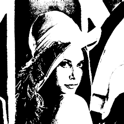
Nota-se uma enorme facilidade de se implementar esse algoritmo no OpenCV. Como visto no primeiro post, para se converter uma imagem colorida em binária é necessário convertê-la para tons de cinza. Isso é feito já na leitura da imagem na linha 13, com o parâmetro IMREAD_GRAYSCALE da função im_read. Todo o trabalho de binarização da imagem é feito em apenas uma linha de código como se vê na linha 23. O resultado desta técnica é a foto abaixo.

Os Melhores Treinamentos sobre Sistemas embarcados e IoT
Cursos com professores qualificados para acelerar sua carreira e projetos
Por ser tão simples, mostrarei como seria feito no SimpleCV. No script digite:
img = Image("lena.png").toGray().binarize(128).invert()
img.show()
img.write("simplecv_lena_threshold.png")
Tudo é feito na primeira linha de código. Lê-se o arquivo, converte para escala de cinza, converte a imagem para binário com o limite de 128. A função invert() serve para inverter pixels 1 para 0 e 0 para 1. Depois exibe e salva a imagem. O resultado é a imagem abaixo. Vale mencionar que as imagens geradas pelo OpenCV e SimpleCV, apesar de muito parecidas, não são iguais.

Figura 2
Algoritmo 2: Ordered dithering
Este algoritmo será implementado usando-se a ferramenta octave. O código fonte é o seguinte:
pkg load image

% Lê arquivo colorigo
img_rgb = imread('lena.png');

% Converte para preto e branco
img = rgb2ycbcr(uint8(img_rgb));
img = img(:,:,1);

% Define matrix de Bayer 8x8
bayer8 = [1 49 13 61 4 52 16 64; 33 17 45 29 36 20 48 32; 9 57 5 53 12 60 8 56; 41 25 37 21 44 28 40 24;
 3 51 15 63 2 50 14 62; 35 19 47 31 34 18 46 30; 11 59 7 55 10 58 6 54; 43 27 39 23 42 26 38 22];

% Tamanho imagem e tamanho matrix
size_image = size(image);
size_bayer = size(bayer8);

% Cria uma matriz do tamanho da imagem real repetindo a matriz de bayer
ts = ceil(size_image ./ size_bayer);
BayerImg = repmat(bayer8, ts);
BayerImg = BayerImg(1:size_image(1), 1:size_image(2));

% Quantizacao. Temos 256 tons de cinza / 64 nivel matriz bayer
Q = double(img) ./ 4;

% Compara imagem original com imagem matriz de Bayer. Pixels com valor >=
% ao matriz de Bayer tem valor 1. Todos os outros 0.
image_binary = Q > BayerImg;
image_binary = image_binary .* 255;

imshow(uint8(image_binary))
imwrite(image_binary, "./octave_lena.png");
No algoritmo acima, usamos uma matriz de bayer 8×8. Replicamos essa matriz ao mesmo tamanho da imagem que queremos processar. Depois comparamos pixel a pixel e atribuímos valores de acordo com o algoritmo, 1 onde o pixel da imagem original é maior que o pixel da matriz de bayer e 0 em todos os outros. O resultado é a imagem abaixo.

Figura 3
Algoritmo 3: Error difusion
Para esta última técnica usaremos o Octave e OpenCV. A implementação no Octave está apresentada a seguir.
pkg load image

img_rgb = imread("lena.png");
img = rgb2ycbcr(uint8(img_rgb));
img = img(:,:,1)

img_size = size(img);
x_max = img_size(1);
y_max = img_size(2);

img = double(img);

for x = 1:x_max,
 for y = 1:y_max,
 % Lê o valor do pixel
 oldpixel = img(x,y);

 % Se maior que 128, atribui nivel 255, senão 0
 if(oldpixel > 128)
 newpixel = 255;
 else
 newpixel = 0;
 end

 % Atribui valor ao pixel na imagem final
 image_floyd(x,y) = newpixel;

 % Calcula erro
 quant_error = double(oldpixel - newpixel);

 % Verifica limites da imagem e acumula erro
 if(x + 1 <= x_max)
 img(x+1,y) = double((img(x+1,y) + 7/16 * quant_error));
 end
 if ((x-1 > 0) && (y+1 < y_max))
 img(x-1,y+1) = double((img(x-1,y+1) + 3/16 * quant_error));
 end
 if(y + 1 <= y_max)
 img(x,y+1) = double((img(x,y+1) + 5/16 * quant_error));
 end
 if((x + 1 <= x_max) && (y + 1 <= y_max))
 img(x+1,y+1) = double((img(x+1,y+1) + 1/16 * quant_error));
 end
 end
end

imshow(image_floyd);
imwrite(image_floyd, "octave_floyd.png");
A imagem gerada pelo código acima é apresentada na figura 4.
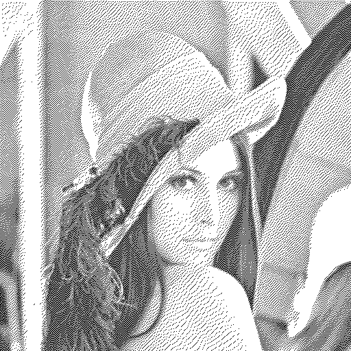
Figura 4
E esta é a implementação no OpenCV:
#include <QCoreApplication>
#include <highgui.hpp>
#include <core.hpp>
#include <imgproc.hpp>
#include <iostream>

using namespace cv;
using namespace std;

int main(int argc, char *argv[])
{
    // Carrega a imagem em preto e brancos
    cv::Mat image = cv::imread("lena.png", cv::IMREAD_GRAYSCALE);

    // Se a imagem não foi carregada, erro
    if(!image.data)
    {
        cout << "nenhuma imagem!";
    }
    else
    {
        // Converte imagem pra float
        cv::Mat img_float;
        image.convertTo(img_float, CV_32FC1);

        cv::Mat image_floyd = cv::imread("lena.png", cv::IMREAD_GRAYSCALE);
        int x_max = image.rows;
        int y_max = image.cols;


        for(int x = 0; x < x_max; x++)
        {
            for(int y = 0; y < y_max; y++)
            {

                // Read pixel value
                float oldpixel = img_float.at<float>(x,y);
                uchar newpixel = 0;

                // check if more than 50//
                if(oldpixel > 128.0f)
                {
                    newpixel = 255;
                }
                else
                {
                    newpixel = 0;
                }

                // set pixel value into new image
                image_floyd.at<uchar>(x,y) = newpixel;

                // calculate error
                float quant_error = (float)(oldpixel - (float)newpixel);

                // Verifica limites da imagem e acumula erro do pixel
                if(x + 1 <= x_max)
                {
                    img_float.at<float>(x+1,y) = (img_float.at<float>(x+1,y) + (float)(0.4375 * quant_error));
                }
                if((x-1 > 0) && (y+1 < y_max))
                {
                    img_float.at<float>(x-1,y+1) = (img_float.at<float>(x-1,y+1) + (float)(0.1875 * quant_error));
                }
                if(y + 1 <= y_max)
                {
                    img_float.at<float>(x,y+1) = (img_float.at<float>(x,y+1) + (float)(0.3125 * quant_error));
                }
                if((x + 1 <= x_max) && (y + 1 <= y_max))
                {
                    img_float.at<float>(x+1,y+1) = (img_float.at<float>(x+1,y+1) + (float)(0.0625 * quant_error));
                }
            }
        }
        cv::imshow("teste", image_floyd);
        cv::imwrite("opencv_floyd.png", image_floyd);
    }

    return 0;
}
A imagem gerada está representada na figura 5 abaixo.

Figura 5
Neste algoritmo, como comentado no post anterior [1], possui uma complexidade maior e por isso um tempo de processamento superior. Primeiro, converte-se o arquivo RGB em tons de cinza. Depois é necessário varrer toda a imagem, e a cada iteração, recalcula-se e acumula-se o erro. Caso o valor do pixel seja acima de 128, atribui-se 255, caso contrário 0. Deve-se destacar que o tempo de processamento no OpenCV é muito menor que no Octave.
Conclusão
Atualmente existem diversas ferramentas para processamento de imagem que são muito robustas e simples. Nos exemplos deste post, nota-se a extrema facilidade de se implementar alguns algoritmos de binarização. O reuso de bibliotecas nos permite aprimorar os algoritmos, deixando-os mais rápidos, robustos e simples de serem usados. Porém deve-se tomar o cuidado de não apenas usar as funções, mas sim entender a teoria por trás dos algoritmos.


